Linear Model Selection and Regularization

Linear Model Selection and Regularization

The linear model has distinct advantages in terms of inference and, on real- world problems, is often surprisingly competitive in relation to non-linear methods. Hence, before moving to the non-linear world, we discuss in this section some ways in which the simple linear model can be improved, by replacing plain least squares OLS fitting with some alternative fitting procedures.

\(Y = \beta_0 + \beta_1 X_1 + \beta_2 X_2 + \dots + \beta_p X_p + \epsilon\) When we should consider alternatives to the OLS?

• For prediction accuracy: in particular when $p>n$, the number of predictors is larger than the number of observation we have high variance, close to overfitting, and so a low prediction accuracy.

• For model interpretability: when we have a lot of predictors, we can have a lot of predictors that are not significative, and so we want to select the most significative predictors and remove the irrelevant ones, by just setting their coefficients to zero.

We will present some mehotds that addresses these problems.

Selection Model Criteria

But first it is worth mentioning some criteria that we can use to select the best model. The $C_p$, AIC, BIC and adjusted $R^2$ are model selection criteria used to assess and compare statistical models based on their fit and complexity

1. ::: definition For fitted least squares model containing $d$ predictors, the $C_p$ is an estimate of test error MSE is: \(C_p = \frac{1}{n} (RSS + 2d\hat{\sigma}^2)\) where $\hat{\sigma}^2$ is an estimate of the variance of the error $\epsilon$[^1]. Essentially, the Cp statistic adds a penalty of $2d\hat{\sigma}^2$ to the training RSS in order to adjust for the fact that the training error tends to underestimate the test error. :::

   As a consequence, the $C_p$ statistic tends to take on a small value for a model with a low test error, and so it is used to select the model with the lowest $C_p$ value.\

2. ::: definition The AIC criterion is defined for a large class of models fit by maximum likelihood. \(\text{AIC} = -2\ln(\mathcal{L}) + 2d\) where $\mathcal{L}$ is the maximized value of the likelihood function for the estimated model, and $d$ is the number of predictors in the model.
   In the case of the least squares model, linear, we have that the AIC is: \(AIC = \frac{1}{n\hat{\sigma}^2} (RSS + 2d\hat{\sigma}^2)\) where $\hat{\sigma}^2$ is an estimate of the variance of the error $\epsilon$. Hence for least squares models, Cp and AIC are proportional to each other. :::

   Including additional variables always reduces RMSE and increases $R^2$, though they are not significative, so the AIC metric penalizes adding terms to a model. The goal is to find the model that minimizes AIC; models with k more extra variables are penalized by 2k.\

3. ::: definition BIC or Bayesian information criteria: similar to AIC with a stronger penalty for including additional variables to the model: \(\text{BIC} = \frac{1}{n} (RSS + \log(n)d\hat{\sigma}^2)\) Like Cp , the BIC will tend to take on a small value for a model with a low test error, and so generally we select the model has the lowest BIC value. :::

4. ::: definition The Adjusted $R^2$ is a modified version of the $R^2= 1 - RSS/TSS$ that has been adjusted for the number of predictors in the model. \(\text{Adjusted } R^2 = 1 - \frac{RSS/(n-d-1)}{TSS/(n-1)}\) :::

   This is because we recall that the RSS decreases as more variables are added to the model, but TSS remain the same, and so the $R^2$ will increase, but the adjusted $R^2$ will decrease if the added variables are not significative.
   
   Remark: Unlike the $C_p$, AIC, and BIC, the adjusted $R^2$ is better when it has a large value, which indicates a model with a small test error.
   
   The intuition behind the adjusted R2 is that once all of the correct variables have been included in the model, adding additional noise variables will lead to only a very small decrease in RSS

Subset Selection

A first group of methods are the so called Subset Selection methods, that are used to select a subset of predictors that are used to fit the model. These are the Best Subset Selection and Stepwise model selection procedures

Best Subset Selection

The Best Subset Selection method fits a separate least squares regression for each possible combination of the $p$ predictors.
That means that we fit the model on all the subset that contains only one predictor, than we fit the model on all the combination subsets that contain two predictors, and so on. For $p=k$ we have $2^k$ possible subsets, and so we have to fit $2^p$ models. The possible combinations are $\binom{p}{k} = \frac{p!}{k!(p-k)!}$.

We can summarize the procedure of the Best Subset Selection in the following algorithm:

::: algorithm ::: algorithmic . Let $\mathcal{M}_0$ denote the null model, which contains no predictors. This model simply predicts the sample mean for each observation.
. (a) Fit all $\binom{p}{k}$ models that contain exactly $k$ predictors. (b) Pick the best among these $\binom{p}{k}$ models, and call it $\mathcal{M}_k$. Here best is defined as having the smallest RSS, or equivalently largest $R^2$.
. Select a single best model from among $\mathcal{M}_0, \ldots, \mathcal{M}_p$ using the prediction error on a validation set, $C_p$ (AIC), BIC, or adjusted $R^2$. Alternatively, use the cross-validation method. ::: :::

Remark: If cross-validation is used to select the best model, then Step 2 is repeated on each training fold, and the validation errors are averaged to select the best value of k. Then the model $\mathcal{M}_k$ fit on the full training set is delivered for the chosen $k$.

Although we have presented best subset selection here for least squares regression, the same ideas apply to other types of models, such as logistic regression. In the case of logistic regression, instead of ordering models by RSS in Step 2 of Algorithm 1, we instead use the deviance.

::: definition The deviance is negative two times the maximized log-likelihood; the smaller the deviance the better the fit. :::

While best subset selection is a simple and conceptually appealing approach, it suffers from computational limitations (when $p$ is large the number of possible models increase rapidly). Best subset selection may also suffer from statistical problems when p is large. The larger the search space, the higher the chance of finding models that look good on the training data, even though they might not have any predictive power on future data.

Stepwise Selection

The enormous search space of the best subset selection can lead to overfitting and high variance of the coefficient estimates. The Stepwise Selection method is a more computationally efficient alternative, it explore a far more restricted set of models.

Forward stepwise selection begins with a model containing no predictors, and then adds predictors to the model, one-at-a-time, until all of the predictors are in the model.
In particular, at each step the variable that gives the greatest additional improvement to the fit is added to the model.

::: algorithm ::: algorithmic . Let $M_0$ denote the null model, which contains no predictors. (a) Consider all $p - k$ models that augment the predictors in $M_k$ with one additional predictor. (b) Choose the best among these $p - k$ models, and call it $M_{k+1}$. Here best is defined as having the smallest RSS or highest $R^2$. . Select a single best model from among $M_0, \ldots, M_p$ using the prediction error on a validation set, $C_p$ (AIC), BIC, or adjusted $R^2$. Alternatively, use the cross-validation method. ::: :::

Unlike the best subset selection, which involves fitting $2^p$ models, forward stepwise selection involves fitting one null model, along with $p-k$ models in the $k$th iteration, for $k = 0, …, p-1$.
This add up to a total of \(1+ \sum_{k=0}^{p-1} (p-k) = 1 + \frac{p(p+1)}{2}\)

[Attention:]{style=”color: red”} with the Stepwise selection method it is not guaranteed to find the best possible model out of all $2^p$ models containing subsets of the $p$ predictors.

Backward Stepwise Selection

The Backward Stepwise Selection is a similar method to the forward stepwise selection, but it starts with the full model containing all the predictors, and then removes the least useful predictors one at a time.

::: algorithm ::: algorithmic . Let $M_p$ denote the full model, which contains all $p$ predictors. (a) Consider all $k$ models that contain all but one of the predictors in $M_k$, for a total of $k-1$ predictors. (b) Choose the best among these $k$ models, and call it $M_{k-1}$. Here best is defined as having the smallest RSS or highest $R^2$. . Select a single best model from among $M_0, \ldots, M_p$ using the prediction error on a validation set, $C_p$ (AIC), BIC, or adjusted $R^2$. Alternatively, use the cross-validation method. ::: :::

As for the Forward Stepwise selection method we have that the Backward Stepwise selection method is computationally faster, since it has to search trough only $1 + \frac{p(p+1)}{2}$ models, so we can use it in settings where $p$ is too large.

[Attention 1:]{style=”color: red”} like the ForwardStepwise selection method it is not guaranteed to find the best possible model out of all $2^p$ models containing subsets of the $p$ predictors.

[Attention 2:]{style=”color: red”} Backward requires that the number of samples $n$ is larger than the number of predictors $p$. This is a requirement for the least squares to be fully fit. In contrast, the forward stepwise selection can be used also when $n<p$.

Choosing the optimal model

How we define which model is the best? The model containing all the predictors will always have the smallest RSS and the largest $R^2$, since these are related to the training error.
But we wish to select a model that has a low test error, not a low training error. In order to select the best model with respect to test error, we need to estimate this test error. There are two way to do this:

1. Since the training error is a sort of estimate of the test error, we can adjust the training error to estimate indirectly the test error, by accounting for the bias due to the overfitting in the training error. Using the $C_p$, AIC, BIC, or adjusted $R^2$.

2. We can directly estimate the test error using the validation set method or the cross-validation method.
   This procedure has an advantage relative to AIC, BIC, $C_p$ and adjusted $R^2$, in that it provides a direct estimate of the test error, and doesn’t require an estimate of the error variance $\sigma^2$ or to know $d$.

In the case of having multiple models (with differnt numbers of variables), that have been proven to be equivalent in terms of the test error, using different approaches(cross-validation, validation set...), we can refer to the one-standard-error rule :

::: proposition We first calculate the SE of the estimated test MSE for each model size, and then we select the smallest model (fewest predictors) for which the estimated test error is within one standard error of the lowest point on the curve (lowest MSE). :::

The reason is that it is best to choose the simplest model to interpret.

Regularization

In the previous section we have seen that the best subset selection and the other methods involve fitting (OLS) a linear model with a subset of predictors. As an alternative, we use a technique that fit a model containing all the $p$ predictors, but it constrains or regularizes the coefficient estimates, or that shrinks them towards zero. This is called Regularization and the methods used are called Shrinkage methods.
It may not be immediately obvious why such a constraint should improve the fit, but it turns out that shrinking the coefficient estimates can significantly reduce their variance

Ridge Regression

We remember from section 1 that the OLS fitting procedure estimates the $\beta_0, \beta_1, \dots, \beta_p$ coefficients by minimizing the RSS: \(RSS = \sum_{i=1}^{n} (y_i - \hat{y}_i)^2 = \sum_{i=1}^{n} (y_i - \beta_0 - \sum_{j=1}^{p} \beta_j x_{ij})^2\) Ridge regression uses a similar approach but it estimates the coefficients by minimizing a different quantity. The ridge regression coefficient estimates $\hat{\beta}^R$ are the values that minimize: \(\sum_{i=1}^{n} (y_i - \beta_0 - \sum_{j=1}^{p} \beta_j x_{ij})^2 + \lambda \sum_{j=1}^{p} \beta_j^2 = RSS + \underbrace{\lambda \sum_{j=1}^{p} \beta_j^2}_{\text{Shrinkage Penalty}}\) where $\lambda \geq 0$ (determined seperately) is a tuning parameter that controls the amount of shrinkage: the larger the value of $\lambda$, the greater the amount of shrinkage. The shrinkage penalty has the effect of shrinking the stimates of $\beta_j$ towards zero. The $\lambda$ parameter is used to control the amount of shrinkage.

Ridge regression will produce a different set of coefficient estimates, $\hat{\beta}{\lambda}^R$ , for each value of $\lambda$. Selecting a good value for $\lambda$ is critical, cross validation is used for this.

[:]{style=”background-color: yellow”} The standard least square coefficient estimates are *scale equivalent*: multiplying $X_j$ by a constant $c$ simply leads to a scaling of the least squares coefficient estimates by a factor of $1/c$. The product $X_j\hat{\beta}_j$ remains the same. The coefficient estimate $\hat{\beta}_j$ simply changes to counteract the scaling in $X_j$, leaving the predictions and interpretation consistent.
In contrast, the Ridge regression coefficent estimatescan change *substantially* when we multiply a predictor by a constant, due to the shrinkage penalty term in the ridge regression formulation upwards. Thus, this means that the $X_j\hat{\beta}{j, \lambda}^R$ will depend on both the value of $\lambda$ and the scaling of the $j$th predictor. Or even on the scale of the other predictors.
Therefore, to bst apply ridge regression we use to standardize the predictors before fitting the model. We use the formula: \(\tilde{x}_{ij} = \frac{x_{ij}}{\sqrt{\frac{1}{n} \sum_{i=1}^{n} (x_{ij} - \bar{x}_j)^2}}\) so that all the predictors have the same scale. Note that the denominator is the estimated standard deviation of the $j$th predictor $\implies$ the standardized predictors standard deviation one.

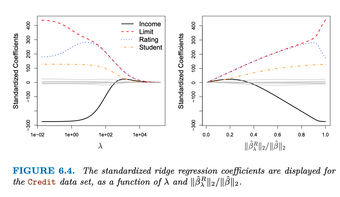{width=”80%”} []{#fig:ridge_regression label=”fig:ridge_regression”}

Ridge regression advantages over OLS

Ridge regression advantages over OLS are rooted in the bias-variance tradeoff:
As $\lambda$ increases, the flexibility (variance) of the ridge regression fit decreases, leading to decreased variance but increased bias. This also reduce the problem of Multicollinearity and reduce the model complexity.

The Lasso

The big drawback of the ridge regression is that it will include all the predictors in the model, and the penalty term will only shrink the coefficients towards zero, but it will not set them to zero. This may not be a problem for prediction accuracy, but it can create a challenge in model interpretation in settings in which the number of variables p is quite large. The lasso is a alternative that overcomes this disadvantage. The lasso coefficients $\hat{\beta_^L}$ are the values that minimize:

\(\sum_{i=1}^{n} (y_i - \beta_0 - \sum_{j=1}^{p} \beta_j x_{ij})^2 + \lambda \sum_{j=1}^{p} |\beta_j| = RSS + \underbrace{\lambda \sum_{j=1}^{p} |\beta_j|}_{\text{Shrinkage Penalty}}\) Where the shrinkage penalty is not squared as in the ridge regression. We can say that the lasso uses an $l_1$ penalty, while the ridge regression uses an $l_2$ penalty. Moreover, the power of the lasso is to shrink some coefficents to zero, when the $\lambda$ is large enough. This means that the lasso can be used for variable selection. As a result, models generated from the lasso are generally much easier to interpret than those produced by ridge regression. We say that the lasso yields sparse models—that is, sparse models that involve only a subset of the variables.

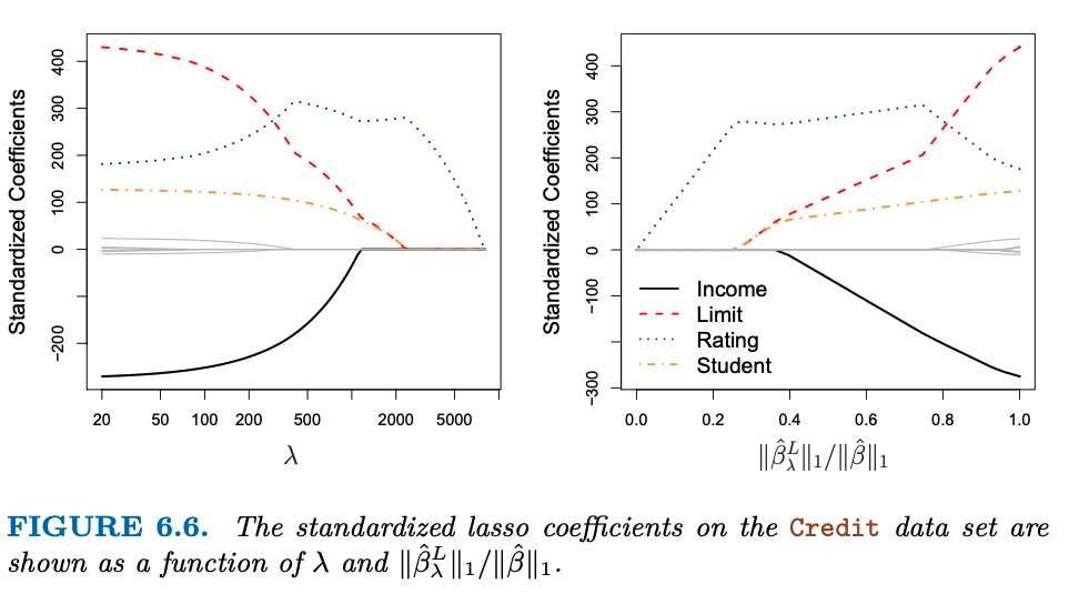{width=”80%”} []{#fig:lasso_regression label=”fig:lasso_regression”}