Deep Learning

Single Layer Neural Networks

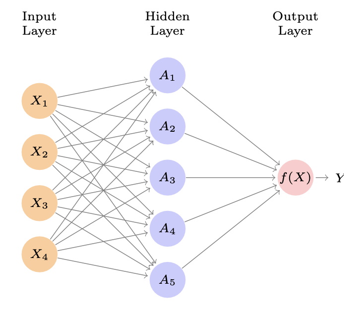
A single layer Neural Network is composed by at least 3 layers: an Input layer, vector of $p$ variables $X_1, X_2, \dots, X_p$, a Hidden layer, and an Output layer, a single variable $Y$. The Hidden layer is composed by $M$ nodes, each node is a linear combination of the input variables $X_1, X_2, \dots, X_p$ and a non-linear function, the activation function $\sigma$. The neural network builds a nonlinear function that predict the output vector, the response, $Y$. It is called single because it has only one hidden layer.

We have already seen some methods for nonlinear prediction, but this is different beacuse of the structure of the model. The image 7.1 shows a feedforward neural network, for modeling a qunatitative response with 4 predictors.
The arrows indicate that each of the inputs from the input layer feeds into each of the $K$ hidden units. The neural network has a mathematical form as: $f(X) = \beta_0 + \sum_{k=1}^{K} \beta_k h_k(X)$

Each layer has a predifined number of units $K$. Eaxh unit is composed of 3 elements:

Two trainable parameters for each input: $w$ as weight and $\beta$ as bias; The coefficient and the intercept.
A nonlinear activation function $g()$.

For an input vector $X = (X_1, X_2, \dots, X_p)$, the output of each $k$th activation unit is: $A_k = h_k(X) = g(\beta_{0k} + \sum_{j=1}^{p} w_{jk}X_j)$ The output vector is $A = (A_1, A_2, \dots, A_K)$.

We can think of each $A_k$ as a different trasformations $h_k(X)$ of the original features.
Then, these $K$ activations from the hidden layer feed into the output layer, resulting in: $f(X) = \beta_0 + \sum_{k=1}^{K} \beta_k A_k = \beta_0 + \sum_{k=1}^{K} \beta_k g(\beta_{0k} + \sum_{j=1}^{p} w_{jk}X_j)$ A linear regression model with the transformed features $A_k$ as predictors.
All the parameters $\beta_{0k}, w_{jk}, \beta_k$ and the weights $w$ are estimated from the data minimizing the squared error loss. The Loss function to minimize in order to estimate the parameters is the already known Mean Squared Error. In the early days of NN the activation function was the sigmoid function: $g(z) = \frac{1}{1 + e^{-z}}$ which is the same function used in logistic regression to convert a linear function into probabilities between 0 and 1. Nowadays, the preferred activation function is the Rectified Linear Unit (ReLU): $g(z) = \max(0, z) = \begin{cases} z & \text{if } z > 0 \\ 0 & \text{if } z \leq 0 \end{cases}$ Although it thresholds at zero, because we apply it to a linear function, the constant term $w_k0$ will shift this inflection point.
In other words, the model : $f(X) = \beta_0 + \sum_{k=1}^{K} \beta_k g(\beta_{0k} + \sum_{j=1}^{p} w_{jk}X_j)$ derives $K$ new features by copmuting $K$ linear combinations of the original features $X_1, X_2, \dots, X_p$ and then squashes them with the activation function $g()$. The final model is a linear regression model with the new features as predictors.

Remark: It is essential that the activation function is a nonlinear function, so the model is a nonlinear model.

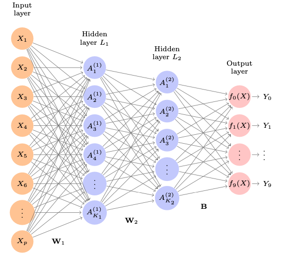
Multilayer Neural Networks

When we have more than one hidden layer we have a Multilayer Neural Network. The model is more complex, but the idea is the same. The model is a linear regression model with the new features as predictors. When adding a new hidden layer, the output of the preceding layer will become the input.

{width=”50%”}

Now, for example, if we want to train a multilayer neural network to a qualitative response, so using the softmax function to convert the output to probabilities: $f_m(X) = P(Y=m | X) = \frac{e^{Z_m}}{\sum_{l=0}^{C} e^{Z_{l}}}$ where $h_j(X)$ is the output of the $j$th unit in the hidden layer. The model is a linear regression model with the new features as predictors. The parameters are estimated by minimizing the negative multinomial likelihood.

, we look for coefficients estimates that minimize the negative multinomial likelihood: $- \sum_{i=1}^{n} \sum_{m=1}^{M} y_{ik} \log (f_m(x_i))$ also known as the cross-entropy loss.

Fitting a Neural Network

So, the easiest way to fit a neural network is to minimize the error function, e.g. the MSE: $\min_{w, \beta_0, \beta_1, \ldots, \beta_p} \frac{1}{2} \sum_{i=1}^{n} (y_i - f(x_i))^2$

where $f(x_i)$ is the output of the neural network: $f(x_i) = \beta_0 + \sum_{k=1}^{K} \beta_k g(\beta_{k} + \sum_{j=1}^{p} w_{jk}x_{ij})$ The goal is to find the couple $(w, \beta)$ that minimizes the error. We can do that using Gradient Descent. Suppose we represent all the parameters in one long vector $\theta = (\beta_0, \beta_1, \ldots, \beta_K, w_{11}, w_{12}, \ldots, w_{Kp})$. Then we can rewrite the objective (7.1) as: $R(\theta) = \frac{1}{2} \sum_{i=1}^{n} (y_i - f_{\theta}(x_i))^2$ The intuition of the gradient descent algorithm is the following: We start with a guess $\theta_0$, we then cevaulate R in that point and we also compute the derivative in that point. If thw values obtained are smaller than the value of the function in the previous point, we move in that direction. We repeat this process until we reach a minimum.

Backpropagation

How do we find and compute this values of $R(\theta)$ and its derivative? The answer is the Backpropagation algorithm. The idea is to compute the derivative of the error function with respect to each parameter. The algorithm is based on the chain rule of calculus.

Basically, we compute the gradient $R(\theta)$ at a timestamp $m$: $\nabla R(\theta^m) = \frac{\partial R(\theta)}{\partial \theta} \bigg|_{\theta = \theta^{(m)}}$

So we compute the derivative in the point $\theta^{(m)}$, this gives us the direction for $\theta$ in which R increases. So we want to move in the /textitopposite direction. We update the parameters as: $\theta^{(m+1)} = \theta^{(m)} - \eta \nabla R(\theta^m)$ where $\eta$ is the learning rate, a hyperparameter that we decide. For small values of $\eta$ the algorithm slowly reduce R: $R(\theta^{(m+1)}) < R(\theta^{(m)})$ The algorithm is repeated until the gradient is zero. Then, we arrived to the local minimum of the function.

Remark: The algorithm does not gurantee the global minimum, but only a local minimum.

The calculation of the gradient in (7.2) is pretty easy thanks to the chain rule since R is a sum, its gradient it’s also a sum over the $n$ observations.

Since $R(\theta)= \sum_{i=1}^{n} R_i(\theta)$, the gradient is the sum of the terms: $R_i(\theta) = \frac{1}{2} (y_i - f_{\theta}(x_i))^2 = \frac{1}{2} \left( y_i -\beta_0 - \sum_{k=1}^{K} \beta_k g (w_{k0} + \sum_{j=1}^{p}w_{kj}x_{ij}) \right)^2$ to simplify the notation we can write $z_{ik} = w_{k0} + \sum_{j=1}^{p}w_{kj}x_{ij}$. So to compute the gradient we first take the derivative with respect to $\beta_k$:

\[\frac{\partial R_i(\theta)}{\partial \beta_k} = \frac{\partial R_i(\theta)}{\partial f_{\theta}(x_i)}\cdot \frac{\partial f_{\theta}(x_i)}{\partial \beta_k} = - (y_i - f_{\theta}(x_i)) \cdot g(z_{ik})\]

And now we take the derivative woth respect to $w_{kj}$:

\[\frac{\partial R_i(\theta)}{\partial w_{kj}} = \frac{\partial R_i(\theta)}{\partial f_{\theta}(x_i)}\cdot \frac{\partial f_{\theta}(x_i)}{\partial g(z_{ik})} \cdot \frac{\partial g(z_{ik})}{\partial z_{ik}} \cdot \frac{\partial z_{ik}}{\partial w_{kj}}= - (y_i - f_{\theta}(x_i)) \cdot \beta_k \cdot g'(z_{ik}) \cdot x_{ij}\]

We notice that in (7.3) and (7.4) we have the same residual term $-(y_i - f_{\theta}(x_i))$. In (7.3) a fraction of this residual is attribuited to each of of the hidden units, according to $g(z_{ik})$. In (7.4) the residual is attribuited in similar way to input $j$ via hidden unit $k$. In other words, the act of differentiating assigns a fraction of the residual to each of the parameters via the chain rule. This process is known as backpropagation.

[]{#sec:appendix label=”sec:appendix”}

Useful Statistics to Remember

We remember here some important statistic relations that are helpful to understand better the meaning of the contents of this document.

Given a estimator $\hat{\theta}$ of a parameter $\theta$ we can say that the Mean squared error of the estimator is: $MSE(\hat{\theta}) = E[(\hat{\theta} - \theta)^2]$
The Bias of an estimator is defined as: $Bias(\hat{\theta}) = E[\hat{\theta}] - \theta$
The Variance of an estimator is defined as: $Var(\hat{\theta}) = E[(\hat{\theta} - E[\hat{\theta}])^2]$
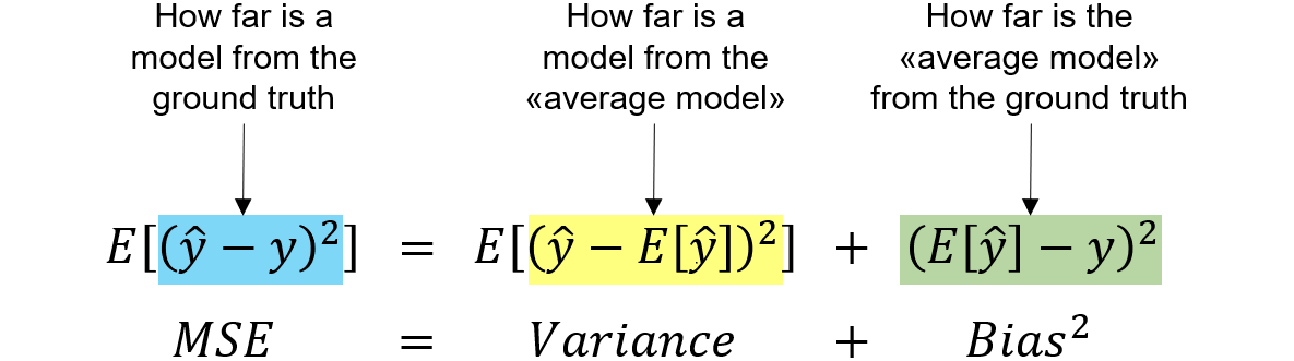
We remember than the importnat relation of the MSE with the Bias and the variance, which is the explanation for the Bias-Variance Tradeoff: $MSE(\hat{\theta}) = Var(\hat{\theta}) + Bias(\hat{\theta})^2$